Trend Views
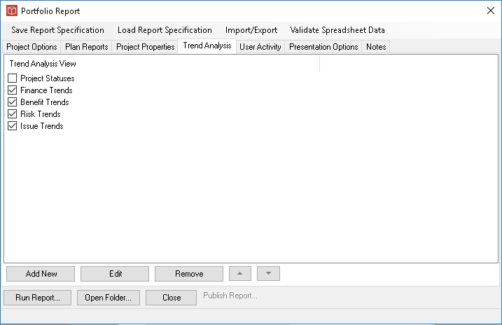
A trend analysis for display or reporting is a complex thing with many options so to save time ins etting them up again and again and to get consistency we use a saved view approach.
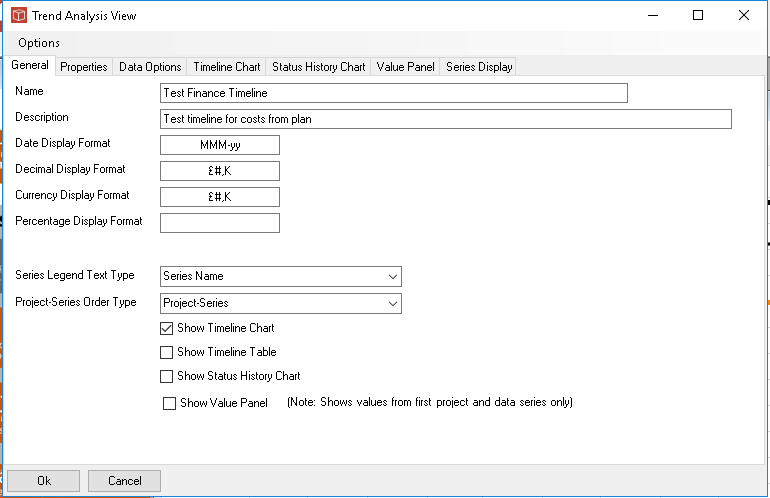
In the Analysis window or the reports you can add a blank view and then either set it up by hand or load in an existing view from the saved views list. You can also remove the views and order them as some reports will display them in their order from the form. By unticking them they will not be used but can be reactiveted easily later. The saved views can also be edited/adjusted if you want and then saved themselves if required. Below we look through the common parts of the form for a trend analysis. In the General tab we can see and alter the Name and Description of the View. If a View is to be saved it will use the name as the view name, Unless you give a new name it will overwrite the existing saved view. Loading a saved view and saving the current view are done in the options menu. You can also save and load the view in XML format from there too. You can also set the formats you want to be used for dates and other data types and then the lick lists below allow you to set the naming of data series and the ordering. These are both particulalry important when working with multiples, especially multiple properties and multiple projects (portfolios). Finally the tick boxes allow you to choose which trend elements should be created under this view, you can select all if you want but it is most likey to be just one in each saved view (or one chart type and the timeline table). Note Value panels only work in project trend analysis.
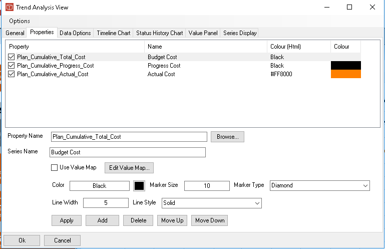
The 2nd tab allows you to select the properties you want to analyse. You can select as many properties as you wish from the database. Select using Browse, set up your colour and line options and then use Add. Of course you can select and edit then Apply if you wish. Also delete and reorder. When each property is only displayed once i.e. in a project analysis you set the line colour options here. If the trend analysis is running in a portfolio mode the colours will come from the final Series Display tab. The series name is the name used in the chart key if selected, this means you can set somehting exactly right for the meaning of the chart.
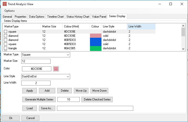
Series display shown here sets the colours for Portfolio presentation you can see here it has been set with 'pairs' of the same colour but one item full line the other dashed. When using a Project/series order type of Project-Series (General tab) and two variables eg budget and spend would give Project A budget and spend in Pink, Project B budget and spend in Blue, project C in green etc.
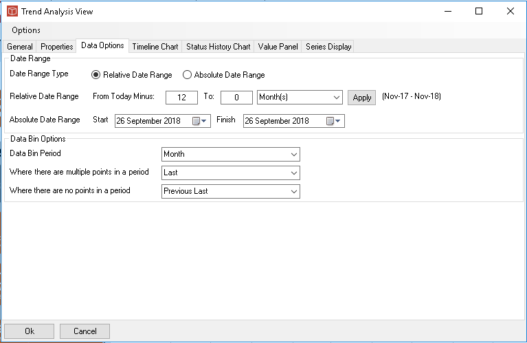
The Data options tab is an important area and applies to all of the analysis types. The data range is usually set to Relative and that applies from today working backwards in the units of time you specifiy. Notice the text far right indicates the range your settings will return, in this example the last 12 months from this month. You can select absolute dates instead although this is less popular. The Bin options control how your data is selected for presentation. Usually for a uniform presentation you will choose a time bin i.e. week, month or year but you can choose no bin (more on that in a minute). This will then prepare a set of data into bins in the example below Nov17-Nov18 monthly, 13 bins. If there was one status change in each of those months then the data set is straightforward. The options below control when there was more than one or none in a particular bin period. Last and Previous Last are the most commonly used options. You can use no binning and the chart will then draw lines directly between each point (in timeline mode) or just show the periods for which data chnges were recorded (in other modes). ometimes you want to see this but usually a chart looks more as you would expect when running a bin period.
Set up of each of the chart types is covered in the following three help pages: |